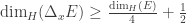
Pinned distance sets using effective dimension

I have just uploaded a paper on the Hausdorff dimension of pinned distance sets. For a given set $E \subseteq \mathbb{R}^n$ , the distance set of E is

$\Delta E = \{ \| x-y\| \mid x,y\in E\}.$

If $x \in \mathbb{R}^n$ , the pinned distance set of E with respect to x is

$\Delta_x E = \{\|x-y\| \mid y \in E\}.$

An important problem in geometric measure theory is to understand the size of $\Delta E$ and, more generally, $\Delta_x E$ . Falconer conjectured that, if $\text{dim}_H(E) > n/2$ , then $\mu(\Delta E) > 0$ . Even in the plane, this is still open (although there has been a recent surge in progress on this question).

In this post we focus on the planar case. Liu showed that, if

$\text{dim}_H(E) = s > 1$

then for “most” (formally defined later) points in the plane,

$\text{dim}_H(\Delta_x E) \geq \frac{4}{3}s - \frac{2}{3}$ .

Shortly thereafter, Shmerkin improved Liu’s result when $s$ is close to 1. Specifically, he showed that if the dimension of E is strictly greater than 1, then

$\text{dim}_H(\Delta_x E) > 0.69$

for most points $x$ .

In this post, I will describe the main argument in my paper on pinned distance sets, where I proved the following.

Theorem 1: If $E \subseteq \mathbb{R}^2$ is analytic and has Hausdorff dimension strictly greater than one, then

$\text{dim}_H(\Delta_x E) \geq \frac{3}{4}$

for all x outside a set of Hausdorff dimension at most one.

Update: It is possible to generalize this bound so that it depends on the Hausdorff dimension of $E$ . In particular, we can conclude that

$\text{dim}_H(\Delta_x E) \geq \frac{\text{dim}_H(E)}{4} + \frac{1}{2}$

The proof of this generalization is essentially the same as the proof of this post, with one or two technical additions. In this post I will sketch the proof of Theorem 1.

The proof of Theorem 1 uses effective dimension. The first part of the proof gives an effective, pointwise, analog of Theorem 1 (this is Theorem 2 below). The second uses a result by Orponen on radial projections and the point-to-set principle to reduce Theorem 1 to our pointwise result. We begin by explaining the proof of the main (effective) theorem.

Theorem 2: Suppose $x, y\in\mathbb{R}^2$ and $e = \frac{y-x}{\|x-y\|}$ satisfy the following conditions.

(C1) $\text{dim}(x), \text{dim}(y) > 1$

(C2) $K^x_r(e) = r - O(\log r)$ for every $r\in\mathbb{N}$ .

(C3) $K^x_r(y) \geq K_r(y) - O(\log r)$ for every $r \in \mathbb{N}$ .

(C4) $K_r(e \mid y) \geq K_r(e) - o(r)$ for every $r \in \mathbb{N}$ .

The main technical result need in the proof of Theorem 2 is a bound on the complexity of projected points, which may be of independent interest. At the conclusion of the next section, we will discuss how this relates to Theorem 2.

1. Projection theorem

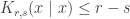
Recall that if $e$ is a unit vector in the plane, the projection of $x$ onto the line spanned by $e$ is

$p_e x = e \cdot x$

As described in a previous post, for every precision r,

$K_r(x \mid p_e x, e) \lesssim K_r(x) - r$

whenever $e$ is random relative to $x$ , i.e.,

$K^x_r(e) \approx r$

Unfortunately, for the application to Theorem 2, we don’t have enough control over e to ensure that e is random relative to x. However, we will have (the weaker condition) that e is random up to precision t, i.e.,

$K^x_s(e) \approx s$

for all $s \leq t$ where

$t \gtrsim \frac{r}{3}$ .

The main content of this section is to show that the techniques for projections developed by Lutz and Stull can be extended to give bounds in this case (at a cost of weakening the bound). Formally, we prove

Theorem 3: Suppose that $\text{dim}(x) > 1$ , $\frac{r}{C} \leq t \leq r$ and $K^x_s(e) \geq s - O(\log s)$ for all $s \leq t$ . Then

$K_r(x\mid p_e x, e) \lesssim K_r(x) - \frac{r+t}{2}.$

The first step in the proof of Theorem 3 is the observation that our previous techniques almost immediately imply the following.

Lemma 4: Suppose r is sufficiently large, $K^x_s(e) \geq s - O(\log s)$ for all $s \leq r-t$ and

$K_{r,s}(x\mid x) \leq r - s$

for all $t \leq s \leq r$ . Then

$K_{r,r,r,t}(x\mid p_e x, e, x) \approx 0$ .

We won’t go into the proof of Lemma 4 in this post. The argument is nearly identical to the one described in this post. We can use Lemma 4 and an oracle reduction idea to show the following.

Lemma 5: Suppose r is sufficiently large, $K^x_s(e) \geq s - O(\log s)$ for all $s \leq r-t$ and

$K_{s,t}(x\mid x) \geq s - t$

for all $t \leq s \leq r$ . Then

$K_{r,r,r,t}(x\mid p_e x, e, x) \approx K_{r,t}(x\mid x) - (r - t)$ .

The point here is to use our oracle construction to get an oracle D so that

$K^D_r(x) \approx K_t(x) + r - t$ .

Then, relative to D, we are able to apply Lemma 4.

We introduce the following definitions. We say an interval [a, b] is yellow if

$K_{s, a}(x\mid x) \gtrsim s - a$

for all $s \in [a, b]$ . We say that [a, b] is teal if

$K_{b, s}(x\mid x) \lesssim b - s$

for all $s\in [a, b]$ . Thus, Lemmas 4 and 5 show that we have tight bound for $K_{b,b,b,a}(x\mid p_e x, e, x)$ on yellow and teal intervals.

1.1 Partition construction

For every t and r, it is not difficult to show the existence of a partition P of $[0, r]$ so that

All intervals in P are either yellow or teal.
All intervals in P are of length at most t
The intervals in P have pairwise disjoint interiors and their union is $[0,r]$ .

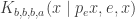
We call a partition satisfying these conditions admissible. Given such a partition, using symmetry of information and Lemmas 4 and 5, we can sum the bounds on each interval in P. This gives the following bound.

$K_r(x\mid p_e x, e) \lesssim \sum\limits_{[a,b]\in P \cap Y} K_{b,a}(x\mid x) - (b - a)\ \ \ \ (1)$ .

Unfortunately, this partition is too naive to immediately imply Theorem 3. To complete the proof, we need to construct a partition which is slightly more optimized.

We say that an interval [a, b] is green if

$b \leq a + t$ , and
$[a,b]$ is both yellow and teal.

Note that, by Lemma 4, if [a, b] is green, then

$K_{b,b,b,a}(x\mid p_e x, e, x) \approx 0$ .

Moreover,

$K_{b, a}(x\mid x) \approx b - a$ .

Thus on green intervals, we maximize the difference

$K_{b, a}(x\mid x) - K_{b,b,b,a}(x\mid p_e x, e, x) \approx b - a$ .

This motivates us to construct a partition of $[0, r]$ which contains many green intervals. In the paper, such a partition is formally constructed. However, for this post, I will elide this details, and skip to the conclusion of Theorem 3.

Proof of Theorem 3: First assume that there is an admissible partition P of [0, r] containing only yellow intervals. Then by the symmetry of information

$K_r(x) \approx \sum\limits_{[a,b]\in P \cap Y} K_{b,a}(x\mid x)$ ,

and so by our previous bound, (1),

$K_r(x) \gtrsim K_r(x\mid p_e x, e) + r$ ,

and the conclusion follows.

If no such partition exists then it is possible to show that there is an admissible partition P of [0, r] satisfying the following: The total length of green intervals in P is at least t, i.e.,

$\sum\limits_{[a,b]\in P \cap G} b-a \geq t.$

Again by the symmetry of information we can conclude that

$K_r(x) \gtrsim t + B + K_r(x\mid p_e x, e)\ \ \ \ (2)$

where

$B := \sum\limits_{[a,b]\in P \cap (Y-G)} b-a$

is the total length of bad intervals (intervals which are yellow, but not green). Therefore, by (1) and (2), we see that

$K_r(x\mid p_e x, e) \lesssim K_r(x) - t - B\ \ \ \ (3)$

Combining (3), and the fact that $K_{b,a}(x\mid x) \lesssim 2(b-a)$ ,

$K_r(x\mid p_e x, e) \lesssim \min\{K_r(x) - t - B, B\},$

from which the conclusion follows.

1.2 Connection between projections and distances

The connection between projections and distances comes from the following fact.

Observation: Let $x, y, z\in\mathbb{R}^2$ , be points such that $\|x-y\| = \|x-z\|$ . Let

$e_1 = \frac{y-x}{\|x-y\|}$ , $e_2 = \frac{z-y}{\|x-z\|}$ .

Then

$p_{e_2} x = p_{e_2} w$ ,

where $w = \frac{y+z}{2}$ . Moreover,

$K^x_s(e_2) \approx K^x_s(e_1)$ ,

for all $s \leq -\log \|y-z\|$ .

To see why this is useful, suppose that $x, y, z$ satisfy the hypothesis of the observation. Then it is not difficult to show that

$K_{r-s}(x \mid y) \lesssim K_{r}(z\mid y) + K_{r-s}(x\mid p_{e_2} x, e_2)$

If, in addition, we assume x is independent of y, this is equivalent to

$K_{r-s}(x) \lesssim K_{r}(z\mid y) + K_{r-s}(x\mid p_{e_2} x, e_2)$

Then, since $s = -\log \|y-z\|$ , it is not hard to see that

$K_r(z\mid y) \lesssim K_r(z) - K_s(y)$ .

Combining these facts, we deduce

$K_{r-2}(x) \lesssim K_r(z) - K_s(y) + K_{r-s}(x\mid p_{e_2} x, e_2)$

Applying our projection result, Theorem 3, with respect to $x, e_2, s, r - s$ ,

$K_{r - s}(x\mid p_{e_2} x, e_2) \lesssim K_{r-s}(x) - \frac{r}{2}$

and so we have

$K_{s}(y) + \frac{r}{2} \lesssim K_{r}(z) \ \ \ \ (4)$

The point of (4) is that it gives strong lower bounds on the complexity of any point $z$ whose distance from $x$ is $\|x-y\|$ . We now describe how to use this in order to prove Theorem 2.

2. Proof of the pointwise analog of Thereom 1

We now turn to the pointwise analog of Theorem 1, which gives a lower bound on the effective dimension of $\|x-y\|$ , whenever $x, y$ satisfy certain conditions.

Theorem 2: Suppose $x, y\in\mathbb{R}^2$ and $e = \frac{y-x}{\|x-y\|}$ satisfy the following conditions.

(C1) $\text{dim}(x), \text{dim}(y) > 1$

(C2) $K^x_r(e) = r - O(\log r)$ for every $r\in\mathbb{N}$ .

(C3) $K^x_r(y) \geq K_r(y) - O(\log r)$ for every $r \in \mathbb{N}$ .

(C4) $K_r(e \mid y) \geq K_r(e) - o(r)$ for every $r \in \mathbb{N}$ .

Then

$\text{dim}^x(\|x-y\|) \geq \frac{3}{4}$ .

In addition to the projection result (Section 1), Theorem 2 relies on the following the general bound, which holds at every precision

$K^x_r(\|x-y\|) \gtrsim \frac{K_r(y)}{2} \ \ \ \ (5)$

The proof of this is very similar to the argument for projections (and is in fact simpler). To keep this exposition short, we will not give a proof of this bound here.

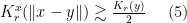
The proof of Theorem 2 combines (5) with our projection result. We first choose precision t so that

$K_t(y)\approx \frac{r}{2}$

Then, by our naive bound (5), we see that

$K^x_t(\|x-y\|) \gtrsim \frac{r}{4}$ .

Thus, by symmetry of information it suffices to show that

$K^x_{r,t}(\|x-y\| \mid \|x-y\|) \gtrsim \frac{r}{2}$

Let D be an oracle (as described previously) which reduces the complexity of y so that

$K^D_r(y) \approx r - \epsilon r$

for some small $\epsilon > 0$ . Let

$z \in B_{2^{-t}}(y)$

and $s = -\log \|y-z\|$ . If s is greater than r/2, then we can use the argument of Lemma 4 to conclude that

$K^D_r(z) > K^D_r(y)$

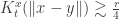
Otherwise, if s is less than r/2, by the bound (4) given in Section 1.2,

$K^D_r(z) \gtrsim K^D_t(y) + \frac{r}{2} \gtrsim r$

Thus, in either case,

$K^D_r(z) > K^D_r(y)$

Therefore, relative to oracle D, if we are given

a $2^{-t}$ approximation of y
a $2^{-r}$ approximation of $\|x-y\|$ , and
x as an oracle

we can compute a $2^{-r}$ approximation of y. Indeed, we simply enumerate all points z with distance $\|x-z\| = \|x-y\|$ such that $K^D_r(z) \leq r - \epsilon r$ . We have just seen that any such point must be within $2^{-r}$ of y, and the claim follows. In the language of Kolmogorov complexity, this is written

$K^x_{r,t}(\|x-y\| \mid \|x-y\|) \gtrsim K^{D,x}_{r,t}(y\mid y)$

By the properties of oracle D, condition (C3), and our choice of t, we can conclude

$K^x_{r,t}(\|x-y\| \mid \|x-y\|) \gtrsim \frac{r}{2} - \epsilon r$

The conclusion follows since $\epsilon$ can be arbitrarily small.

3. Reduction to pointwise analog

To finish this post, we now describe how to use Theorem 2 to prove the main theorem of the paper, Theorem 1.

Theorem 1: If $E \subseteq \mathbb{R}^2$ is analytic and has Hausdorff dimension strictly greater than one, then

$\text{dim}_H(\Delta_x E) \geq \frac{3}{4}$

We begin by noting (using well known facts of geometric measure theory) that it suffices to show Theorem 1 for the case when E is compact, and

$0< \mathcal{H}^s(E) < \infty$

for some s > 1. Let $\mu = \mathcal{H}^s\vert_{E}$ .

The main result used in the reduction is the following theorem of Orponen on radial projections. For any x, define

$\pi_x(y) = \frac{y-x}{\|x-y\|}$

The pushforward measure of $\mu$ is the measure defined by

$\pi_{x\#}\mu(S) = \mu(\pi_x^{-1}(S))$

for any subset S of the unit circle. Orponen’s theorem implies the following.

Theorem: There is a Borel set B with Hausdorff dimension less than 1 such that, for all $x \in \mathbb{R}^2 - B - spt(\mu)$ ,

$\pi_{x\#}\mu$ is absolutely continuous with respect to $\mathcal{H}^1 \vert_{\mathcal{S}^1}$

We can use this theorem in our reduction by combining it with recent results in algorithmic information theory. Specifically, let A be an oracle relative to which E is effectively compact and $\mu$ is lower semicomputable. Then it is possible to show that, for any x,

The set of directions e such that $K^{x, A}_r(e) < r - O(\log r)$ infinitely often is of measure zero.
The set of points y in E such that $K^{x, A}_r(y) < K^{x,A}_r(y) - O(\log r)$ infinitely often is of $\mu$ measure zero.

Facts (1) and (2), combined with Orponen’s theorem, show that, for every x outside a set B of dimension at most one, there is some y in E so that (x,y) satisfies conditions (C1)-(C4) of Theorem 2, relative to oracle A.

We can conclude Theorem 1 by applying the point-to-set principle for this choice of A and using Theorem 2. Since $E$ is effectively compact relative to $A$ , it is not difficult to show that $\Delta_x E$ is effectively compact relative to $(x, A)$ , for every point $x$ . A theorem of Hitchcock shows that, for every $x$ ,

$\text{dim}_H(\Delta_x E) = \sup\limits_{y\in E} \text{dim}^{x,A}(\|x-y\|)$

Thus, for every $x$ outside B, by taking any $y \in E$ so that $x, y$ satisfy (C1)-(C4) relative to $A$ , and applying Theorem 2,

$\text{dim}_H(\Delta_x E) \geq \frac{3}{4}$

and the proof is complete